The sections of this chapter introduced the concept of pointers and all the operators needed to work with them and dynamic memory. Pointers and their operators are a recurring theme we encounter throughout most of the remaining chapters of the text. But, it is often easier to understand abstract concepts like pointers with a concrete use. So, before we end the chapter, let's look at two detailed, albeit simplified, examples to help solidify the pointer concept and syntax.
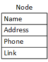
Programmers use pointers and dynamic memory allocation to create dynamic or linked data structures. The names describe a data structure constructed with dynamic memory allocated on the heap and linked with pointers, making both appropriate. Figures 1 and 2 illustrate two examples of these structures: linked lists and binary trees. Programmers call the large boxes in the examples nodes, and the arrows represent pointers called links. C++ programs implement nodes as objects instantiated from structures (the next chapter) or classes. Nodes contain the data we wish to store in the structure and one or more pointers linking them together. The "data" may span a broad spectrum of complexity - anything from a single data element like a character to thousands of complex data elements.
Programmers can implement dynamic data structures and their nodes in many ways. For example, a node can embed the data or have a pointer to a separate structure containing the data. Lists can be sorted (e.g., alphabetically) or unsorted. The link in the last list node may be nullptr or point to the first node in the list. A list may have links pointing in one direction or two. Binary trees can be balanced (keeping the left and right sides about the same height) or unbalanced. Sometimes, binary trees are back-threaded with pointers from the nodes back up the tree. When using dynamic structures, programmers always match the structure's behaviors with the problem they are solving.
Embedded Data
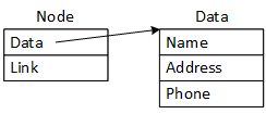
Pointer To Data
Two node options. By "handcrafting" nodes for specific problems, programmers can embed data in the node or save a pointer to it. They can generalize the data structures (enable them to manage any data) by separating the organizing and data operations. Programmers can generalize the pointer version by making the link a void pointer: void*. The text elaborates void pointers in a subsequent chapter. Templates, detailed in Chapter 13, offer a more elegant solution.
A linked list. Sometimes, programmers replace arrays with linked lists, so comparing their behaviors is understandable. Four specific operations illustrate the relative advantages and disadvantages of the two data structures.
Asscessing a specific data item with a known location. Arrays are much faster than linked lists.
Searching for a specific value. Arrays may be a little faster than linked lists, but not a great deal.
Inserting and removing data. Inserting data into an array, Figure 4 generally takes much more time than inserting it into a linked list, Figure 5. The time for removing data is comparable to inserting it.
Memory utilization. If a program creates a large array but only uses a small portion, it wastes most of the memory. Worse, if the array is too small, the program can run out of space because it can't enlarge it. If the program replaces the small array with a new, larger one, it pays a time penalty for copying the saved data from the old to the new one.
Programmers must match a data structure's strengths and weaknesses to a given problem. When a problem uses an operation frequently (e.g., inserting data into the structure), programmers choose a structure with a fast insertion operation. Programmers can "afford" structures with slower operations when the problem uses them infrequently.
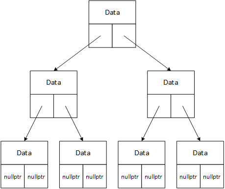
A binary tree. Each binary tree node contains data and links pointing to the left and right sub-trees. This organization makes it possible to search the tree very quickly. If a binary tree contains a million nodes and is well-balanced, programs can search for a specific node by examining no more than twenty nodes (i.e., the tree is at most twenty levels high).
Inserting data into an array. It is easy to add new data at the end of an array, but it is necessary to first "make a hole" to insert data into a partially filled array. The insertion process begins at the bottom of the array and works upward toward the insertion position. During each iteration, it moves the last element down one position. Then, it moves the next element into the vacated position. This process continues from the bottom up until there is a vacancy at the insertion point, where it inserts the new data. If each data item is large or the array contains many data items, this shifting operation becomes expensive in the amount of time it takes.
Inserting data into a linked list.
The data is wrapped in a new node created with new
The link in the new node is set to point to the node following the insertion point
The link in the node preceding the insertion point is set to point to the new node
Recall that an address is an integer, so steps 2 and 3 are just integer assignment operations, among the fastest computer operations. Contrast this animation with the animation in Figure 4.
We conclude with a few simplified code fragments implementing a linked list append operation. The code illustrates some of the pointer operators introduced in the chapter. The code is a brief introduction and may seem mysterious now, but it will become understandable as you continue your studies. The following statements assume the program has a class named node that has:
A data field represented as a single variable: char data;.
A link field, implemented as a pointer to a node: node* link;.
Appending a new node at the end of a list. Appending a node is a special, simple case of the more general insertion problem illustrated in Figure 5. The new data's address is stored in the pointer variable d (perhaps a function parameter) as the code fragment begins.
The program creates the first list node, named list, as an automatic variable. The program "holds on to" list and uses it to access all the list data.
Many list operations, for example (e), require programmers to initialize the link field in the first node.
The ellipses represent the program adding nodes to the list.
The statement initializes variable l (lowercase L) to point to the first node in the list. The program uses the variable to "walk the list" (i.e., follow the links from the first to the last node).
The loop finds the last node in the list. It begins with l pointing to the first list node and continues while the link in that node is not nullptr. The program advances l to the next node in the list with the assignment statement.
The last four statements, (f) through (i), implement the append operation. The first creates a new node to hold the data.
The statement stores the data in the new node.
The statement sets the new node's link to nullptr, indicating it is the new list end.
l points to the current last list node. The program updates its link to point to the new last node.
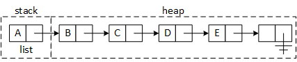
The memory layout of the list created in Figure 6. The first node in the list, named list, is allocated as an automatic variable on the stack. The program dynamically allocates the remaining nodes on the heap with new. The "ground" symbol shown in the last node's link field is an alternate way of indicating the link contains nullptr.
for (node* l = &list; l != nullptr; l = l->link)
	cout << l->data << endl;
Displaying all the data in a list. Sequentially examining each data structure node is called "walking," and examining a specific node is called "visiting." So, to display all the data in a list, we walk the list and visit each node.