Computer scientists use the term "dynamic" to describe actions that occur during program execution. So, dynamic data structures are containers that store application data and exhibit two dynamic traits. First, programs construct them from blocks of memory dynamically allocated on the heap using the new operator and linked together with pointers. Second, the pointers allow the structures to dynamically organize the data they store, arranging it to increase the efficiency of one or more access operations. C++ implements most of the containers in its Standard Template Library (STL) (introduced later in the chapter) as dynamic data structures. Despite the many dynamic data structures in use, most share a core set of operations, though they may use different names that better reflect the structure's behavior.
create the data structure; done with a constructor in C++.
destroy the structure when it is no long needed; done with a destructor in C++.
insert a new data item in the structure. The operation's name varies (e.g., add, append, push, etc.), reflecting how the structure organizes the stored data. The operation may or may not allow duplicate data.
search for a given data item. Programmers also refer to this operation by various names, including "get," "find," and "peek," among others. Searching is a specialized form of the more general access operation. It is appropriate for associative data structures (defined below), like binary trees, and is the term used throughout their discussion.
remove an existing data item from the structure.
Standard dynamic data structure operations.
Although these operations are common across most data structures, their implementations vary substantially depending on how the structure organizes the data it stores.
Binary trees (aka binary search trees) are one of many dynamic data structures. They are sufficiently complex to illustrate some advanced programming features while remaining simple enough for beginning computer scientists to follow their fundamental behavior. If the trees are balanced (wide and bushy rather than tall and skinny), the insert and search operations are relatively fast, with a run order or Big O of O(log n). The text uses them here to demonstrate two versions of a data structure based on one and two template variables.
Associative Data Structures
associative data structure, associative search, orderable, key, comparator, functor, CList
Generally, data structures organize data independently of the data's type and access individual data items by their position in the structure. Programs search associative data structures for a key. A key is a portion of the stored data, and if the program locates the key in the structure, it can access all the associated data. For example, if the structure stores instances of the Person class and searches for a person's name, it can retrieve all data associated with that person. Binary trees order or organize the data they store, enabling fast searches but requiring the data to be relatively orderable. The following description and subsequent binary tree implementations assume that the data stored in the tree can be ordered and compared with the < and == operators, respectively. The fundamental types order naturally with the less-than operator - 5 < 10 - and compare with the equality operator - 10 == 10. However, objects in a tree require a different ordering mechanism. Programmers can overload the relational operators for the class whose objects the tree stores, or they can create a comparator. Programmers can implement comparators as functions passed as argument by pointer, or as functors (objects the act like functions).
To lay a foundation for presenting the binary tree operations, we need to extend our computer science vocabulary, and revisiting some data structures we've studied previously is helpful. A stack typically only allows a program to access the data at a single position, the stack's top, making the insert (push), search (peek), and remove (pop) operations relatively fast, but also limiting the problems stacks can solve. Arrays are more flexible, allowing programs to access any array element with an index in the range 0 .. size-1, making the search operation relatively fast. Inserting new data at the end of a partially filled array or removing data from the end are also fast operations, but are slow and tedious operations at other positions (see Inserting data into an array). Linked lists improve the insert and remove operations but slow the search. Most linked lists access data by its position in the list. However, we saw with the CList that it is possible to access list data with a key, which is how binary trees operate.
Binary trees are self-organizing data structures, meaning that they manage their internal organization independent of the client program. For example, if the client enters the same data into two trees in different orders, the trees may have distinctly different shapes, which are beyond the client's control. Binary tree implementations typically make the pointers that bind the tree private and don't provide any getters, completely isolating or hiding the data organization from the client and making access by position impossible. Consequently, clients storing data in binary trees must access it with a key. Trees are an example of a sub-category of data structures called associative data structures - structures that associate one data value, the key, with another data value. When a "natural" association exists between the key and the other value, we can implement an associative data structure with one template variable; otherwise, we need at least two variables.
Name
Address
Dilbert
225 Elm
...
Alice
256 N 400 W
...
Wally
718 Washington
...
Asok
633 Adams
...
Word
mirror
rabbit
cat
queen
Count
8
27
12
22
(a)
(b)
Visualizing template variables with tables.
Although binary trees organize data differently from arrays, making them appear and behave quite differently, we can use tables to help understand how template variables work when performing tree operations.
This example illustrates a structure storing Employee data. Each column represents one class member variable (the ellipses stand for any number of additional members), and each row represents one stored object. Name and address form part of the stored information describing an individual, making them "naturally" associated with that information. A client program could use a name as a search key without storing additional information in the tree. If a search finds a key, it returns the entire row, making all the associated information available to the client. We can solve this problem with a binary tree based on a single template variable.
Some solutions require mapping a key to a value where the only association between the two is a specific problem. For example, imagine the problem of counting all unique words in a book. The words form the keys, while the counts represent the data. Outside the problem, words and counts are not naturally associated. We can solve this problem by creating a class with two members, word and count, and storing instances of the new class in a binary. Alternatively, we can solve it with a binary tree using two template variables. We'll revisit this problem later in the chapter.
If we handcraft the search and remove functions for a specific problem, we can make the key any data type. However, a general, library-grade solution is more restrictive. Using a single template variable requires making the key the same type as the stored data. Typically, the client creates a partially filled object for the key, including only enough information to satisfy the equality operation. Imagine that a tree stores instances of an Employee class as illustrated in (a). An appropriate key object is an instance of Employee with only the Name variable filled. Searching for part of the stored data is called an associative search. We can relax the restriction on the key type by using two or more template variables.
Binary Tree Specification And Images
template, binary tree, Tree class
template <class T>
class Tree
{
    private:
               T data;
        Tree<T>* left;
        Tree<T>* right;
 . . .
};
(a)
(b)
(c)
A binary tree and the operational pointers.
A single binary tree element, represented by the squares in the illustrations, is called a node. Computer scientists typically draw trees upside down and refer to the node at the top as the root. The root node may contain data or serve only as the tree's "handle" (i.e., the variable a client program defines to access the tree). The following descriptions and examples implement the latter version, simplifying some operations at the expense of others, and imply that a logically "empty" tree consists of a single root node with no data. The Greek letter lambda (λ) is an abbreviation for nullptr.
A basic template binary tree class with three member variables: data holds the data stored in the node, while the left and right pointers link to the node's subtrees, building and organizing the tree structure.
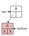
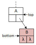
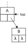
This figure and those following illustrate each tree node as a square with the data member at the top and the left and right pointers on the bottom. Arrows and λ characters indicate valid and null pointers.
This binary tree arbitrarily inserts the first data item to the root's right subtree and never uses its left pointer. The search and insert operations require a "key" data value provided by the client program. The search operation seeks the "key," and the insert operation attempts to insert it into the tree. As they descend the tree, both operations choose between the left and right subtrees based on the "key:" if key less than the data in the current node, go left; otherwise, go right. In the illustrations, "A" precedes (comes before) "B," and "C" succeeds (comes after) "B." The search operation uses a single pointer, bottom, to indicate the current node. The insert operation uses two pointers, top and bottom, that are moved down the tree so that they are always one level apart. Using two pointers makes it convenient for the operations to access the members of both nodes.
Illustrating Binary Tree Algorithms
binary tree
A C++ binary tree implements operations 1 and 2, create and destroy, with a constructor and destructor, respectively. These operations are algorithmically simple and illustrated with working code in the next sections. The following figures outline operations 4, 5, and 6 (insert, search, and remove), which are more algorithmically complex. The working examples in the following sections demonstrate some optional operations, including a list function.
(a)
(b)
(c)
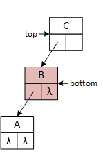
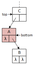
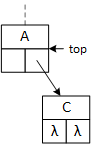
Descending the tree: searching and inserting.
When a program searches for or inserts a node in a binary tree, it descends the tree from the top down. Searching requires one pointer, bottom, while insertion requires both top and bottom. As the operations descend the tree, they compare two data values: the key and the data stored in the bottom node, updating the pointers as they descend the tree. If the key value is less than the bottom node value, the program follows the left subtree; otherwise, it follows the right subtree. Although top and bottom change as the functions descend the tree, this always points to the root node.
The search function begins by initializing the bottom pointer, while the insert function initializes both pointers as illustrated:
Tree<T>* top = this;
Tree<T>* bottom = right;
The operations continue descending the tree and updating the pointers. The operations assume that the stored data supports the == and < operators, which are valid for the fundamental types but require programmers to overload them for class types. This version of the insert operation does not permit duplicate key values in the tree.
while (bottom != nullptr)
{
    if (bottom->data == key) // return the matching data already in the tree
        return &bottom->data;
    top = bottom;									// insert only
    bottom = (top != this && key < bottom->data) ? bottom->left : bottom->right;	// insert
    bottom = (key < bottom->data) ? bottom->left : bottom->right;			// search
}
If the insert operation reaches the bottom of the tree without finding a match, it creates a new node, stores the key data in it, and inserts it into the tree. The second statement assumes that the saved data supports the assignment operation, requiring programmers to overload the assignment operator for "complex" classes (see simple and complex classes). The last statement selects the left or right subtree for insertion. The conditional operator's first sub-expression compares the key to the current or bottom node. The operator's second and third expressions produce pointers to the left and right subtrees. Therefore, the conditional operator produces a valid l-value for the left-hand side of the assignment operator, setting the appropriate subtree to bottom.
bottom = new Tree;
bottom->data = key;
bottom = (top != this && key < bottom->data) ? bottom->left : bottom->right;
Although the remove operation doesn't significantly contribute to the template demonstration, it does illustrate a situation programmers frequently encounter while implementing data structures: some operations are efficient and relatively straightforward, while others are not. Searching for and inserting nodes in a binary tree is an efficient process requiring relatively little code. Removing a node from a binary tree is neither efficient nor straightforward. Computer scientists typically decompose the removal operation into three distinct cases. In the first case, the node selected for removal is a leaf without subtrees. In the second case, the selected node has one subtree. Finally, the node has two subtrees in the third (last) case.
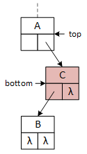
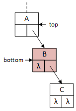
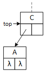
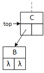
The following figures focus on developing algorithms, leaving the coding to the implementation sections. The figures consistently use a set of features: First, the top and bottom pointers begin at the top of the tree and descend it as described above. Second, the dashed line suggests that the part of the tree above the top pointer doesn't affect the removal algorithm. Third, arrows and λ's represent significant pointers; empty subtree boxes may be null or point to subtrees without affecting the algorithm. Fourth, the figures color the node selected for removal red. Finally, single alphabetic characters represent the stored data, demonstrating a valid insertion order and labeling the nodes.
Case 1.1
Case 1.2
Before Removal
After Removal
Before Removal
After Removal
The remove operation: Leaf (no subtrees).
A binary tree removes a leaf by pruning it and setting the appropriate subtree in its parent (the top node) to null.
Case 2.1
Case 2.2
Case 2.3
Case 2.4
Before Removal
Before Removal
Before Removal
Before Removal
After Removal
After Removal
After Removal
After Removal
The remove operation: One subtree.
The pictures are similar, suggesting that they represent four sub-configurations of case 2: the node selected for removal, bottom, has one subtree, either the left or right subtree. It's either the left or right subtree of its parent, top. The binary tree removes the bottom node and sets the appropriate top subtree to point to the removed node's one subtree.
Case 3
Before Removal
After Removal
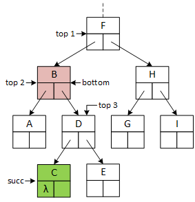
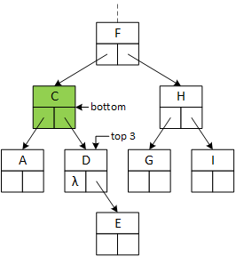
The remove operation: Two subtrees.
The more extensive illustration suggests that removing a node with two subtrees is the most complex case. The removal algorithm progresses in four distinct phases:
Identify a node for removal, shaded red, using the top (labeled "top 1" in the illustration) and bottom pointers to descend the tree. The algorithm can't prune the removal node, as in case 2, because it can't move the node's two subtrees to a single parent subtree.
Locate the removal node's successor (the node with the next highest data value). Informally, it finds the successor by "going right once, then left until it finds a null." The algorithm must "remember" the removal node, making bottom unavailable for the next step, so it introduces a third operational pointer named succ (labeled "succ 1), initialized to bottom's right subtree. It could introduce a fourth pointer, but top is available and reinitialized to bottom (represented by top 2). The algorithm descends the tree, keeping succ and top one level apart. The second phase ends when the algorithm locates the successor, shaded green, with the pointers at the locations labeled "succ 2" and "top 3."
Copy the successor's data (green) node to the removal (red) node, overwriting and replacing the removal node's contents.
Destroy the original successor (green) node using case 1 or 2 as appropriate.