 |
#include <iostream>
#include <iomanip>
using namespace std;

int main()
{
    int    nrows;
    int    ncols;

    cout << "Number of rows: ";
    cin >> nrows;
    cout << "Number of columns: ";
    cin >> ncols;

    int**    table = new int* [nrows];		  // (1)

    for (int i = 0; i < nrows; i++)		  // (2)
        table[i] = new int[ncols];

    for (int row = 1; row <= nrows; row++)
        for (int col = 1; col <= ncols; col++)
            table[row-1][col-1] = row * col;	  // (3)

    for (int row = 0; row < nrows; row++)
    {
        for (int col = 0; col < ncols; col++)
            cout << setw(4) << table[row][col];   // (3)
        cout << endl;
    }

    for (int i = 0; i < nrows; i++)		  // (4)
        delete[] table[i];
    delete[] table;

    return 0;
} |
| (a) | (b) |
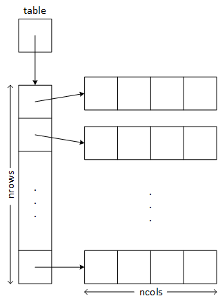
- table is a pointer to a pointer (i.e., it's a pointer with two levels of indirection as illustrated in b.1). table points to an array of row pointers. Each row pointer points to an array that serves as one table row.
-
- The program defines table as
int**, meaning that it is a pointer to a pointer. The data typeint*means that each element of table is a pointer to an integer, that is, an array of integers. - The program must create each table row individually.
- One of the advantages of creating a two-dimensional array as an array or arrays is that the "client" or main-logic code can continue to use the two-index notation: table[row][col].
- The program must individually delete the rows and then the array of pointers. The square brackets, [], inform delete that it is operating on an array.
- The program defines table as